


Access full report
Oops! Something went wrong while submitting the form.

🤍

Facilitated by The Modern Data Company in collaboration with the Modern Data 101 Community
Latest reads...

.png)

.jpg)
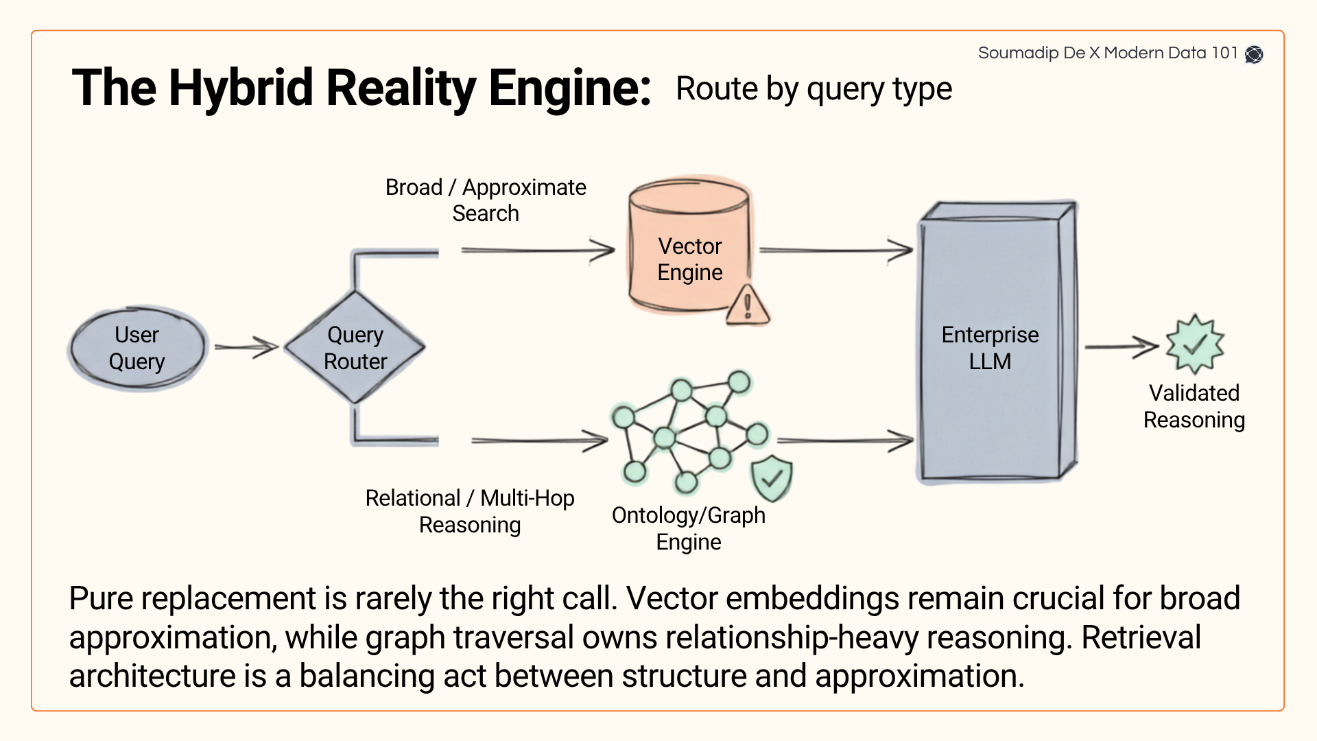

TABLE OF CONTENT


TOC
- Introduction
- A practical perspective to the new reform in the “Shortest Path
- Understanding the “Sorting Step:” The Process
- Understanding the Heap & the Bucket: The Tech
- Shortest Path from Data to Insights (& Actions): Drawing the Parallel
- Shortest Path Architecture When Translated to Big Data Systems
--- Core Principle
--- Components (each exists to reduce distance)
--- Algorithm Parallels / Architecture Specifics
- Zooming Into Some Algorithm Parallels / Architecture Specifics
--- Finding Pivots
--- Bounded Multi-Source Shortest Path
- Architecture at a Glance
Researchers have finally found a faster way to run Dijkstra’s shortest path algorithm: something people thought couldn’t really be improved in a meaningful way. The paper, “Breaking the Sorting Barrier for Directed Single-Source Shortest Paths,” is a breakthrough for Modern Systems which still use a 70-year-old algorithm to “travel from point A to point B.”
For decades, the “bottleneck” in Dijkstra’s algorithm has been the priority queue (the structure that decides which node to process next). The best known limit was O(m + n log n), where log n comes from sorting-like operations inside that queue. It was assumed this was the limit, that we couldn’t beat the “sorting barrier.” (We’ll dive into what this means soon!)
Now, the team found a clever new data structure that avoids that sorting overhead. Their algorithm runs in O(m log^(2/3) n), meaning the log factor is strictly smaller than before.
In simple terms:
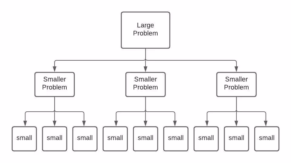
At the risk of oversimplifying, we’ll say that it turns out the new improvement is an application of an even older problem-solving approach laid down by René Descartes in the 17th Century:
Breaking down complex problems into smaller, independent units and solving each to tackle higher-order complex solutions. This approach was formalised by the early philosopher and came to be known as deductive reasoning.

When you use Google Maps to find the fastest route, behind the scenes, it’s running some version of Dijkstra’s algorithm. That’s been the standard way to compute “shortest paths” since the 1950s.
The thing is, even though computers got faster, the mathematical speed limit of the algorithm itself never really improved in a big way. The “sorting step,” deciding which road to explore next, always slowed things down.
The researchers figured out how to skip that slow sorting step with a totally new kind of data structure. That means:
Imagine you’re in a city, trying to find the quickest route from your home to every other place.
Think of standing at an intersection with a clipboard. You mark the distance to every place you’ve discovered. Now, you need to always pick the place closest to you so far to continue exploring.
The problem: every time you pick the next place, you have to shuffle and re-sort your entire clipboard to see which one is smallest. It’s like carrying a stack of maps and constantly re-ordering them by distance over and over again every time you take a step. That’s the “sorting step.” It slows you down.
Instead of one clipboard you keep re-sorting, the researchers built something more like a set of buckets or shelves.
Breaking down into Smaller Problems: Places aren’t all dumped into one big pile that needs sorting. They’re grouped into “zones” or “layers” based on how far they are.
When you explore, you don’t need to shuffle the entire pile. You just go to the shelf that holds the next nearest batch and grab from there. On top of that, they use a graph decomposition trick, like breaking the city map into neighbourhoods. This lets them search locally inside smaller sections, so you don’t pay the full overhead everywhere at once.
In Summary,
- Dijkstra = always re-sorting a messy pile of distances.
- New method = shelves + neighbourhoods → no messy re-sorting, just pick the right shelf and move.
- The result: less wasted motion, less overhead, faster pathfinding.
For spatial clarity, imagine a librarian vs. a warehouse worker.
Dijkstra’s librarian
Every time a new book comes in, they re-order the entire library just to know what’s the next book on the list.
New algorithm’s worker
Tosses books into pre-labelled shelves. No reordering needed. Just check the right shelf when you need the next book.
They replaced decades of “re-sorting” with a smarter “bucketed map of shelves.”
Imagine a librarian who has a big pile of returned books. Each book has a tiny sticker showing how far away its shelf is. Every time a book is returned, the librarian puts it into the giant pile.
To reshelve the “nearest” book, they must re-sort the entire pile to see which one has the smallest distance sticker. After placing that book back, they repeat: re-sort the whole pile again, pick the next nearest, walk there, reshelve. This works, but it’s exhausting: constant sorting, sorting, sorting.
That’s basically Dijkstra: keep the priority queue (the pile) always sorted, so you can pick the closest (extract-min).
They never actually sort the whole pile at once (that would be too expensive). Instead, they keep the pile in a special shape (a heap) so that picking the smallest book is always efficient (log n cost). But every time a new book comes in, the pile has to be slightly reorganised to keep that “always ready” property. That little shuffle is the hidden “sorting tax” that piles up across the whole process.
Now imagine a clever head librarian redesigns the system: Instead of one huge pile, they create buckets of shelves labelled by distance ranges.
When a book is returned, the librarian drops it straight into the right bucket. No big re-sorting. To find the next nearest book to shelve, the librarian just checks the first non-empty bucket. Within that bucket, there might be a small handful of books to order, but it’s way quicker than reordering the entire pile.
Plus, the library is divided into neighbourhoods (wings). Each wing has its own little bucket system. That means sorting effort is split into smaller local problems, not one giant universal problem.
Instead of carefully rebalancing the pile every time, they slap on a quick, cheap label and toss the book into the correct bucket. The rules are simple:
When it’s time to grab the nearest book, you just check the first non-empty bucket. Inside, there may be a little bit of re-checking, but nowhere near the heavy “maintain perfect order” tax of the old system.
So the librarian now spends way less energy moving things around, and the job gets done faster overall.
A heap is like a tree-shaped pile of numbers (distances in Dijkstra).
An example
Say we have distances: [3, 7, 5, 9, 11]
The heap would look like this (as a binary tree)
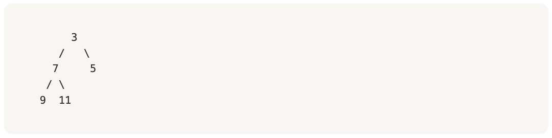
3 is the root (as smallest always on top). 7 ≥ 3, 5 ≥ 3, 9 ≥ 7, 11 ≥ 7 → rule satisfied. 5 is on the right but smaller than 7 on the left (which is allowed). The heap doesn’t care about perfect left-to-right sorting (only needs parents smaller than children).
Extract-min (pop the top)
Take out the root (3). Then move the last element (11) to the root and “bubble it down” to restore order:
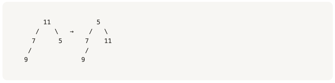
Now 5 is the root (the next smallest). This bubbling costs ~log n steps because you move down the tree.
Insert (add new distance)
Drop the number at the bottom, then “bubble it up” if it’s smaller than its parent. Cheap, but also ~log n in the worst case.
Decrease-key (update distance if you find a shorter path)
Move that node upward until the parent rule is satisfied. Also cheap (can be O(1) in Fibonacci heaps).
Every time you need the “next closest node,” Dijkstra does extract-min. That’s log n work. Over n nodes, that’s n log n total. That’s the sorting tax.
As simple as it may sound, it’s buckets!
Reusing the same distances [3, 7, 5, 9, 11] we see how the new bucket-style method would look compared to the heap.
Say we make buckets of size 5:
Bucket 0-4: (for distances 0 to 4)
Bucket 5-9: (for distances 5 to 9)
Bucket 10-14: (for distances 10 to 14)
Now drop each number into its correct bucket:
Bucket 0-4: [3]
Bucket 5-9: [7, 5, 9]
Bucket 10-14: [11]
Notice: no sorting inside the whole set. Just a cheap throw into the right basket step.
In Dijkstra, we always want the smallest distance next. Here, we simply check buckets in order: First bucket with items is 0-4 → grab 3.
That was O(1): no bubbling, no log n.
Now we check the next non-empty bucket: Bucket 5-9 has [7, 5, 9].
Which one is smallest? Here you might do a tiny local scan → pick 5.
Then the bucket becomes [7, 9].
Next from that same bucket is 7. Then 9. Finally, we check Bucket 10–14 → grab 11.
And you’re done.
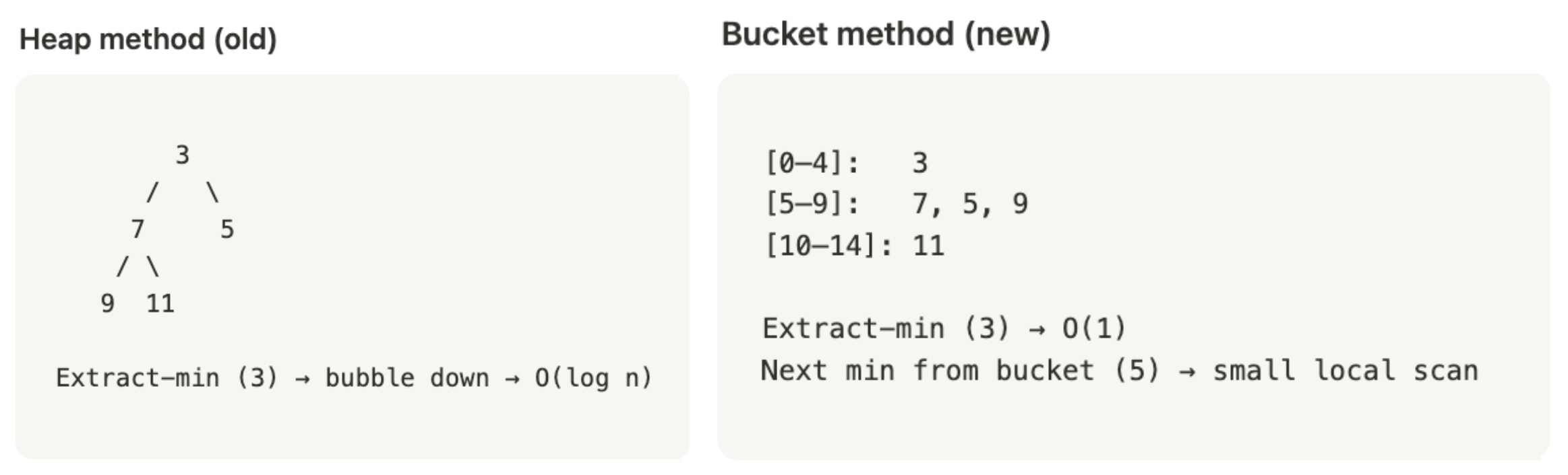
Over huge graphs, these local scans add up to less than the repeated bubbling. That’s why complexity drops from log n per extract to log^(2/3) n overall.
The metaphor transfers really well into the way data products are built and consumed. Think about the old Dijkstra way (heap) in a data org:
Every query, every dashboard, every ML pipeline pulls from a giant shared priority queue: the data lake, the warehouse, the central models.
To deliver an answer, the system constantly has to “bubble up” the right thing by re-sorting across everything. It’s powerful, but it’s expensive. Governance, catalogs, lineage, all trying to keep one mega-pile in order.
Now imagine the new algorithm (bucket system) as a data product ecosystem, or what we have called a modular data ecosystem:
In other words:
Heap world: monolithic data platforms where every new request re-stirs the pot.
Modular world: data product ecosystems where domain buckets keep things lean, composable, and quick to pick from.
It’s a neat parallel, the breakthrough is basically saying: stop forcing global re-sorting, start designing buckets of local context.
That’s exactly the tension data product leaders are feeling: do we keep centralising and paying the governance tax, or do we reorganise into buckets where the next “minimum distance” for the business is easier to grab?
Here’s the model-first, bucket-routed architecture that makes the shortest path from data to insight real and mirrors the new Dijkstra breakthrough.
Note: In all following text, when we say “nearest distance,” we aren’t talking about physical data distances, we mean contextual distance. Just like language models convert sentences to numeric embeddings to calculate the nearest distance and determine similarities.
A data product is “nearer” to a business edge when its semantics, metadata, and context are already aligned with the edge’s “purpose”/goals/specs. The ecosystem detects which buckets (data products) lie “closest” to that purpose and routes the request there first, just as the improved Dijkstra’s algorithm sorts paths into buckets and reaches the shortest one without scanning the entire field.
Deterministic proximity is the principle that, in a well-architected data product ecosystem, the "closeness" of a data product to a business edge (where action happens) is not random or exploratory. It is predictable, measurable, and context-driven. In other words, the ecosystem knows which bucket (data product) is most relevant for a given business question because the semantics (purpose, metadata, lineage, usage context) are embedded directly into the product.
This ensures that the "nearest" insight is always surfaced without trial-and-error, just like an improved algorithm finds the nearest node faster. It shifts the effort from "searching widely" (trial, querying, joining, guessing) to "selecting narrowly" (context guides you directly to the right data product).
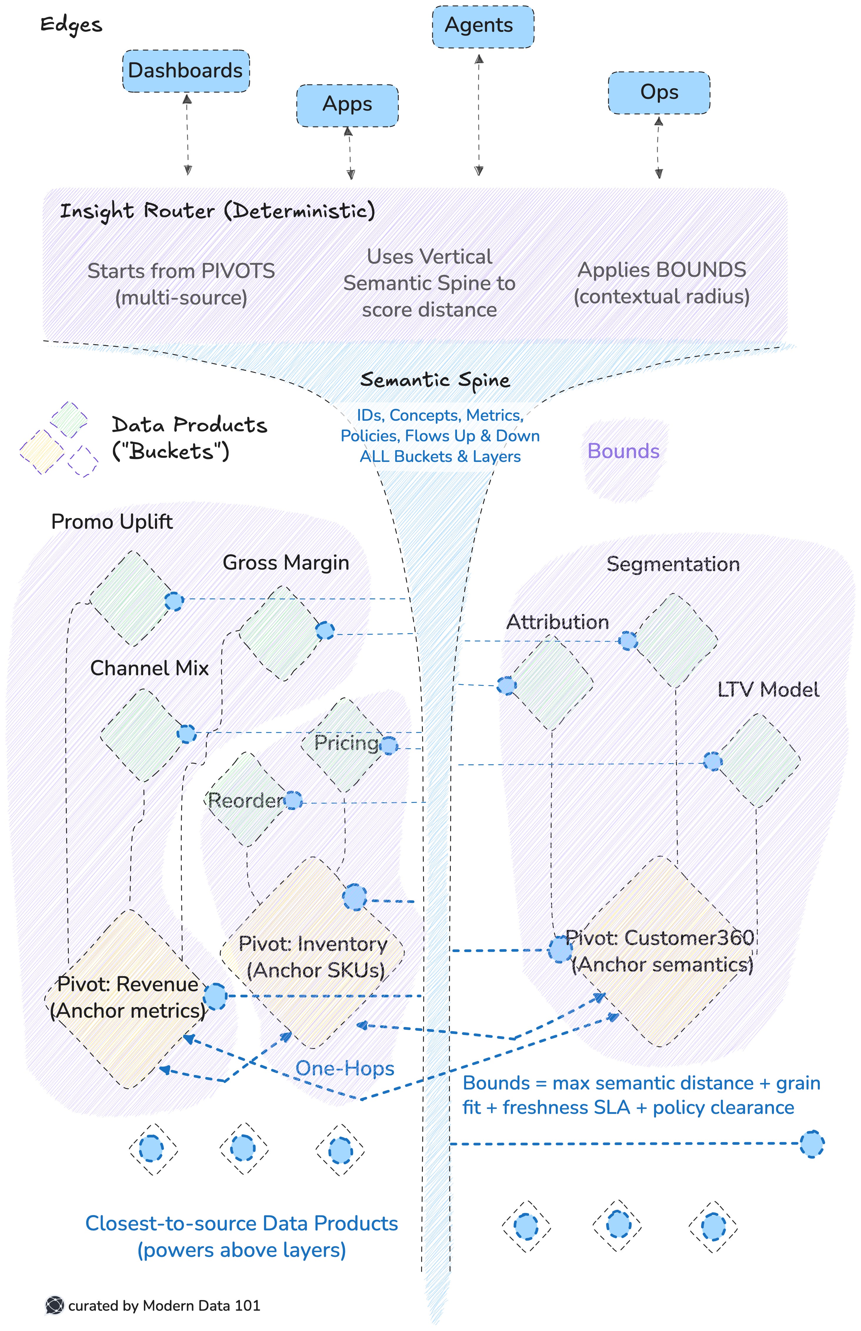
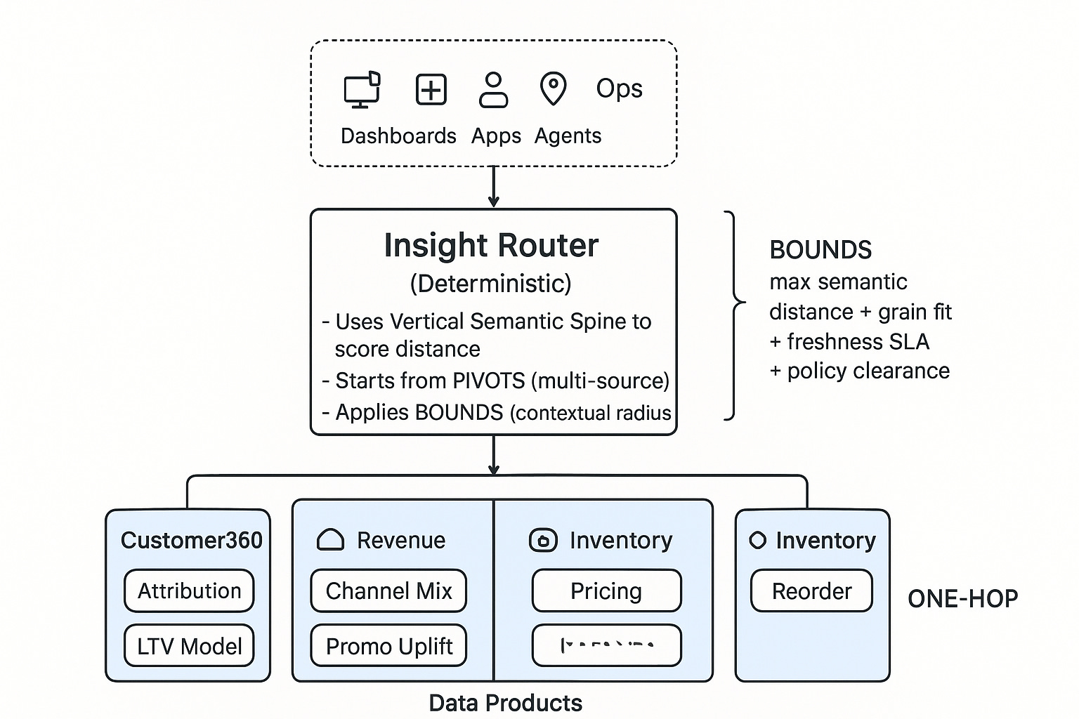
Data products are buckets with brains: each holds its model, data, semantics, and metadata. A vertical semantic spine stitches shared meaning (IDs, concepts, metrics) through every bucket. An insight router picks the nearest bucket deterministically, avoiding global re-sorting.
A question arrives → the router scores buckets using the vertical spine’s semantics → it picks the nearest bucket → execution happens locally → if needed, the spine guides one-hop pulls from adjacent buckets → the answer surfaces at the edge.
No global scan. No cross-org reshuffle. Minimal hops.
Old world: one global heap (central catalog) constantly rebalanced to find the next “smallest” insight, organisational log-n tax.
New world: bucketed priority. Questions are routed to distance-based shelves, with local selection and neighbourhood traversal only.
Graph decomposition = domain buckets; priority bucketing = distance bins; deterministic routing = fewer global operations.
“APAC revenue last 7 days by channel?” → Revenue bucket is nearest (right model, right grain, fresh) → executes locally → one hop to Customer360 only if channel taxonomy needs alignment → answer ships.
Shortest path achieved by bucketed priority + neighbourhood hops, not by central re-sorting. Net effect: you replace platform friction with deterministic proximity.
In Section 3 of the paper, Breaking the Sorting Barrier for Directed Single-Source Shortest Paths, titled “Main Result,” the researchers zoom in on two algorithms:
These are key to understanding the applications and understanding how pillars of Data Ecosystem’s Engine, such as the Insight Router, operate at scale.
Instead of scanning every possible node globally, the algorithm chooses a few special nodes called pivots that act like “checkpoints.” From these pivots, distances to other nodes can be structured more efficiently, reducing global re-sorting.
Think of pivots as landmarks in a city. If you know how far you are from the train station, city hall, and the central park, you don’t need to measure the distance to every building individually. These pivots let you triangulate quickly.
In the modular or data product ecosystems, pivots are anchor products that hold high-value, widely-used semantics, like Customer 360, Revenue, Inventory.
The algorithm doesn’t just start from one node; it launches searches from multiple sources (like several pivots at once). But it sets bounds (limits) so the search doesn’t blow up. You only explore “close enough” neighbourhoods.
Imagine you’re hungry and check Google Maps. Instead of searching all restaurants in the city, it starts from multiple hubs near you (mall, office, home) and only shows those within, say, a 3 km radius. You get results much faster without being overwhelmed.
In the data ecosystem, this means:
So the nearest bucket is discovered not by brute force, but by bounded, multi-source exploration.
Note that this multi-point reference is essential for rich results, data is only good when well connected across touchpoints. It paints a pattern.
Finding Pivots → defines anchor data products that act as semantic landmarks for the ecosystem.
Bounded Multi-Source Shortest Path → enables the insight router to explore only the closest neighbourhoods of buckets, not the whole ecosystem.
A question comes from the edge. The router first orients itself around pivot products (Customer, Revenue, Inventory). Using the vertical semantic spine, it bounds the search only to buckets contextually close to the question. The nearest bucket is selected deterministically. Execution happens locally; if needed, a one-hop to an adjacent bucket finalises the answer.
Pivots give your ecosystem reference points. Bounded multi-source search keeps queries local and efficient. Together, they ensure the “shortest path to insight” works exactly like the new algorithm: no global re-sorting, only smart, bounded neighbourhood discovery.
How to read this:
Finding Pivots → Anchor Products: accelerates orientation; avoids system-wide scans.
Bounded Multi-Source Search → Local Neighbourhoods: explores only close enough buckets; no global re-sorting tax.
Deterministic Proximity → Predictable Routing: the same question always resolves to the same nearest bucket under the same context.
Thanks for reading Modern Data 101! Subscribe for free to receive new posts and support our work.

Find me on LinkedIn 🙌🏻

Find me on LinkedIn 🤝🏻

Find me on LinkedIn 🫶🏻
Join the Global Community of 10K+ Data Product Leaders, Practitioners, and Customers!
Connect with a global community of data experts to share and learn about data products, data platforms, and all things modern data! Subscribe to moderndata101.com for a host of other resources on Data Product management and more!
A few highlights from ModernData101.com
📒 A Customisable Copy of the Data Product Playbook ↗️
🎬 Tune in to the Weekly Newsletter from Industry Experts ↗️
♼ Quarterly State of Data Products ↗️
🗞️ A Dedicated Feed for All Things Data ↗️
📖 End-to-End Modules with Actionable Insights ↗️
Managed by the team at Modern
Your Copy of the Modern Data Survey Report
Better decisions start with shared insight.
Pass it along to your team →
Your Copy of the Modern Data Survey Report
Better decisions start with shared insight.
Pass it along to your team →


Find more community resources
Modern Data 101 is a movement redefining how the world thinks about data. A community built by the same team behind the world’s first data operating system, Modern Data 101 sits at the intersection of data, product thinking, and AI. Spread across 150+ countries, the community brings together a global network of practitioners, architects, and leaders who are actively building the next generation of data systems.
At its core, Modern Data 101 exists to simplify the journey from raw data to tangible and observable impact. It advocates high-potential data systems and next-gen architectures to unify and activate insights and automation across analytics, applications, and operational workflows at the edge.
In a world shifting from data stacks to AI ecosystems, Modern Data 101 helps teams not just navigate the change but lead it.

Find all things data products, be it strategy, implementation, or a directory of top data product experts & their insights to learn from.
Connect with the minds shaping the future of data. Modern Data 101 is your gateway to share ideas and build relationships that drive innovation.
Showcase your expertise and stand out in a community of like-minded professionals. Share your journey, insights, and solutions with peers and industry leaders.


